BUILDING YOUR FIRST MACHINE LEARNING MODEL
From zero to a working predictive model in one focused session. Learn data loading, exploration, train/test splits, model training, evaluation, and the most common mistakes that sink beginners.
By Liyam Flexer · Published Jun 10, 2026 · 14 min read
You are about to train your first machine learning model that actually works on new data.
This is the single most important skill in applied AI. Not the fanciest algorithm. Not the biggest GPU. The ability to take a messy real-world problem, turn it into clean data, train a model, honestly measure how well it will perform in the future, and explain the result.
We will build a house price prediction model — the classic starting project that appears in every serious practitioner’s toolkit.
What You Will Actually Build
By the end of this guide you will have:
- Loaded and explored real (or realistic) data
- Created a proper train/test split
- Trained a linear regression model (the best possible starting point)
- Evaluated it with meaningful metrics and visuals
- Identified the next improvements you would make
Everything is designed so you can copy the code and run it immediately.
Prerequisites (Keep It Minimal)
You need Python 3.9+ and these packages:
pip install pandas scikit-learn matplotlib seaborn jupyter
That is genuinely all you need for a powerful first model.
Step 1: Load and Inspect the Data
We will use a clean synthetic dataset that mimics real house price data (size, bedrooms, distance to city center, etc.). In real life you would load a CSV from your company or a public source like Kaggle.
import pandas as pd
import numpy as np
from sklearn.model_selection import train_test_split
from sklearn.linear_model import LinearRegression
from sklearn.metrics import mean_absolute_error, mean_squared_error, r2_score
import matplotlib.pyplot as plt
import seaborn as sns

# Create realistic synthetic data
np.random.seed(42)
n = 1000

data = {
    'sqft': np.random.normal(1800, 600, n).clip(600, 4500),
    'bedrooms': np.random.randint(1, 6, n),
    'distance_to_center': np.random.normal(12, 8, n).clip(0.5, 45),
    'age': np.random.normal(25, 18, n).clip(0, 90),
}

df = pd.DataFrame(data)
# Generate target with realistic noise and interactions
df['price'] = (
    180 * df['sqft'] +
    25000 * df['bedrooms'] -
    8500 * df['distance_to_center'] -
    1200 * df['age'] +
    np.random.normal(0, 38000, n)   # realistic noise
).clip(85000, 1250000)

print(df.head())
print(df.describe())

You should see relationships across features. The target (price) has a wide range. This is normal. Your job is to find the patterns that explain most of that variance.
Step 2: Quick Visual Exploration
Never skip this. Plots reveal problems and opportunities that summary statistics hide.
# Correlation matrix
plt.figure(figsize=(8, 6))
sns.heatmap(df.corr(), annot=True, cmap='RdYlGn', center=0)
plt.title("Feature Correlations with Price")
plt.show()

# Key relationship
plt.figure(figsize=(8, 5))
sns.scatterplot(data=df, x='sqft', y='price', hue='bedrooms', alpha=0.6)
plt.title("Price vs Size (colored by bedrooms)")
plt.show()

Strong positive relationship between size and price. Color by bedrooms shows the expected vertical stacking. Distance to center should show a negative slope.
Watch: The Intuition Behind What We Are Doing
VIDEO — ANIMATED FOUNDATION
This 8-minute video will make everything that follows feel obvious. The red line “learning” where to sit is exactly what our code will do.
Step 3: Choose Your Algorithm (Start Simple)
We will use Linear Regression as our first model.
Why? Because it is the correct baseline. Read the deep explanation here: Linear Regression Concept and the full set of five essential algorithms: 5 Essential Machine Learning Algorithms.
If a linear model performs terribly, we will know the relationship is highly non-linear and we can reach for trees later.
Step 4: The Train / Test Split (Non-Negotiable)
This single line of code is what separates real machine learning from statistics theater.
X = df.drop('price', axis=1)
y = df['price']

X_train, X_test, y_train, y_test = train_test_split(
    X, y, test_size=0.2, random_state=42
)

print(f"Training on {len(X_train)} examples, testing on {len(X_test)}")
The test set must remain completely untouched until the very end. Touching it earlier is the #1 way beginners fool themselves.
Step 5: Train the Model
model = LinearRegression()
model.fit(X_train, y_train)

print("Coefficients:")
for feature, coef in zip(X.columns, model.coef_):
    print(f"  {feature}: {coef:,.0f}")
print(f"Intercept: {model.intercept_:,.0f}")
Step 6: Evaluate Honestly
Now we finally look at the test set.
y_pred = model.predict(X_test)

mae = mean_absolute_error(y_test, y_pred)
rmse = np.sqrt(mean_squared_error(y_test, y_pred))
r2 = r2_score(y_test, y_pred)

print(f"Mean Absolute Error: ${mae:,.0f}")
print(f"Root Mean Squared Error: ${rmse:,.0f}")
print(f"R² Score: {r2:.3f}")
Interpretation guide:
- MAE tells you the typical error in dollars.
- R² tells you what fraction of the variation in price your model explains (0.8+ is usually strong for this type of problem).
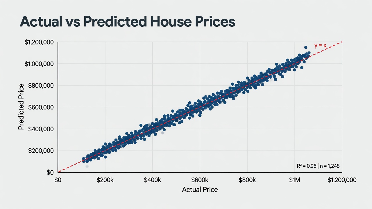
Plot y_test against y_pred. Points should cluster tightly around the diagonal line. Fanning out or curves = your model is missing something important (interactions, non-linearity).
plt.figure(figsize=(8, 6))
plt.scatter(y_test, y_pred, alpha=0.5)
plt.plot([y_test.min(), y_test.max()], [y_test.min(), y_test.max()], 'r--', lw=2)
plt.xlabel("Actual Price")
plt.ylabel("Predicted Price")
plt.title("How Well Did We Do on Unseen Data?")
plt.show()
Watch: Seeing the Same Idea in a Decision Tree Context
VIDEO — HOW TREES APPROACH THE SAME PROBLEM
After you finish the linear model, watch this. You will immediately understand why trees can capture interactions that a straight line misses.
Step 7: Iterate Like a Professional
A first model is never the final model. Good next experiments:
- Add polynomial features for size (non-linear effect of very large or very small homes)
- Create interaction features (sqft × distance_to_center)
- Try a Random Forest or Gradient Boosting model and compare MAE directly
- Remove or cap extreme outliers in the training data only
Document every change and the resulting test-set MAE. This log becomes your most valuable artifact.
Common Beginner Mistakes (Avoid These)
Mistake 1: Evaluating on the training data
You will get beautiful numbers that mean nothing.
Mistake 2: Data leakage
Using information that would not be available at prediction time (e.g. using future averages, or the target variable itself in features).
Mistake 3: Skipping visualization
Numbers lie. Plots reveal whether your model is systematically over- or under-predicting in certain regimes.
Mistake 4: Jumping straight to the fanciest algorithm
XGBoost on day one usually means you never understood why the simpler model failed.
The Mental Model That Actually Matters
Machine learning is not magic. It is automated pattern finding with honest out-of-sample testing.
The code above is less than 30 lines. The thinking — what question am I actually trying to answer? What would “good” look like in dollars or lives saved? How will I know when the model is no longer trustworthy? — is the real work.
Continue Your Journey
- Deepen your understanding of the algorithms: 5 Essential Machine Learning Algorithms Explained Simply
- Master the theory behind the first model you built: Linear Regression
- Explore the full landscape: Machine Learning Concepts
- See how these ideas fit into the bigger AI picture: Artificial Intelligence Hub
You now have a repeatable process that works for almost any tabular prediction problem. The rest is practice, better data, and ruthless honesty about what the numbers actually mean.
Welcome to machine learning. Build something useful today.
Do I need to know advanced math to build useful ML models?+
No. You need solid intuition about what the model is doing and how to interpret its mistakes. The math becomes important later when you need to debug why a model is failing or choose between algorithms.
Why is the train/test split so important?+
A model that has already seen the data it is being tested on will appear to perform perfectly while failing completely on new examples. The split simulates the real world where future data is unseen.
Should I start with linear regression or a more powerful model like XGBoost?+
Always start with the simplest reasonable model (usually linear or logistic regression, or a shallow tree). It establishes a baseline, reveals data issues quickly, and is far easier to debug and explain.
What is the single most common mistake beginners make?+
Training and evaluating on the same data, or leaking information from the test set into the training process (data leakage). Both produce wildly optimistic results that collapse in production.
How long should my first project take?+
If you follow this guide, you can have a working end-to-end model with evaluation in under two hours. The real learning happens when you iterate and try to improve it.